一、概述
1.1 二轴机械臂


1.2 参数识别概述

二、动力学模型


三、力矩测量
伺服电机一般为三个环控制,从底到高排序为电流环,速度环和位置环,电流环都需要使用,其余两环根据需要和设置模式选择使用。
四、参数(线性)分离
参数分离需要参考最小惯性集相关内容
关节的速度和加速度都是通过差分获得,但差分会导致噪声被严重放大,一般来说通过位置差分获得速度噪声还在可接受范围内,再差分计算加速度的话噪声几乎会淹没掉有用的信号。


五、计算速度
采集的数据只有角度信息,因此速度通过中心差分法计算获得
差分,又名差分函数或差分运算,差分的结果反映了离散量之间的一种变化,是研究离散数学的一种工具,常用函数差近似导数。

qf为低通滤波后的角度数据,k为时间序号,T为数据采集时间间隔(此处为1ms)。
%% BLOCK 2
%This program describes the procedure to compute the joint velocity
%estimates using the central difference algorithm given in equation (21)

%First joint velocity estimation (V1)
V1(1) = 0.0;
V2(1) = 0.0;
for j=2:l-1
   V1(j)=(qf1(j+1)-qf1(j-1))/(2*T);
   V2(j)=(qf2(j+1)-qf2(j-1))/(2*T);
end
V1(l) = V1(l-1);
V2(l) = V2(l-1);

%Set velocity vectors as row vectors
V1 = V1';
V2 = V2';
六、数据滤波
数据通过低通滤波器进行处理,过滤高频噪声。
此处用到低通滤波有两处,一为对采集的关节角度使用fir低通滤波器,另一处为对代入位置和速度的模型进行滤波。
低通滤波(Low-pass filter) 是一种过滤方式,规则为低频信号能正常通过,而超过设定临界值的高频信号则被阻隔、减弱。
6.1 角度信息fir低通滤波
使用零相移滤波器filtfilt避免低通滤波产生的时延
%% BLOCK 1
%Filter coefficients
N = 30; % Order
Fc = 0.07; % Cutoff Frequency
flag = 'scale'; % Sampling Flag
win = nuttallwin(N+1); % Create the window vector
b = fir1(N, Fc, 'low', win, flag);% Coefficients using the FIR1 function.

%Filtering for q1 and q2 using the filtfilt function
qf1 = filtfilt(b,1,q1);
qf2 = filtfilt(b,1,q2);
6.2 对代入位置和速度的模型进行滤波
低通滤波函数
f(s)=λ/(s+λ)
λ为截止频率,式4.1通过低通滤波后为
![]()
采集数据为离散数据,因此需要对低通滤波的传递函数(连续)进行处理,使其满足离散信号的滤波,使用zero-order holder可以将连续的低通滤波信号变为离散信号。
零阶保持器(zero-order holder)的作用是在信号传递过程中,把第Tn时刻的采样信号值一直保持到第Tn+1时刻的前一瞬时,把第Tn+1时刻的采样值一直保持到Tn+2 时刻,依次类推,从而把一个脉冲序列变成一个连续的阶梯信号。因为在每一个采样区间内连续的阶梯信号的值均为常值,亦即其一阶导数为零,故称为零阶保持器。
Matlab:将具有连续采样时间的输入信号转换为具有离散采样时间的输出信号。
zero-order holder的传递函数为
G0(s)=(1−e−Ts)/s
通过zero-order holder的低通滤波传递函数为,设g(s)=sf(s)g(s) = sf(s)g(s)=sf(s)

其Z变换为
Z变换(英文:z-transformation)可将时域信号(即:离散时间序列)变换为在复频域的表达式,它在离散时间信号处理中的地位,如同拉普拉斯变换在连续时间信号处理中的地位。

参考Z变换和拉式变换转换为

因此,式5.1的Z变换为
[gD(z)Ya+fD(z)Yb]θ=fD(z)τ
%% BLOCK 4
%This program allows to implement filter (18) and then compute Yaf, Ybf and
%the elements of tau_f given in equation (12)

lambda = 30; %Cut-off frequency

%Coefficients for g(z) in (24)
A1=[1 -exp(-lambda*T)];
B1=[lambda -lambda];

%Coefficients of f(z) in (23)
A2=[1 -exp(-lambda*T)];
B2=[0 1-exp(-lambda*T)];

%Calculus of Yaf and Ybf given in (14)(16)
for i=1:2
    for j=1:9
        Yaf(:,:,i,j) = filter(B1,A1,Ya(:,:,i,j));
        Ybf(:,:,i,j) = filter(B2,A2,Yb(:,:,i,j));
    end
end

%Calculus of the elements of tau_f given in (12)
tf1 = filter(B2,A2,tau1);
tf2 = filter(B2,A2,tau2);
七、参数识别
7.1 识别框架

● On-line
On-line为驱动器-机械臂部分,通过PD闭环(位置和速度)使用力矩控制机械臂,并将输出力矩和关节角度发送到Off-line。
● Off-line
Off-line为计算机处理部分,对接收到的角度数据进行低通滤波,然后通过差分计算速度。将角度,速度和力矩代入模型中,通过滤波后通过参数识别算法获得动力学参数。
参数识别时需要控制机械臂按一定激励轨迹运动,该轨迹会影响参数识别效果,此处输入激励为

其中w1=π(rad/s),w2=0.4π(rad/s)
s设计激励轨迹的目的是为了降低矩阵Yr的条件数。可参考:Jan Swevers et al. Optimal Robot Excitation and Identification, IEEE Trans. on Robotics.
机械臂控制必需确保采用PD闭环控制,保证采集数据的可靠性。
7.2 Matlab实现
流程

程序
%Data loading
clear all
clc
load data01.mat

time = 10;   %Experiment time
T = 0.001;   %Sampling period
l = time/T;  %Number of samples

q1=exps.signals(1,1).values(1:l,1); %Joint position 1
q2=exps.signals(1,2).values(1:l,1); %Joint position 2
u1=exps.signals(1,3).values(1:l,1); %Voltage 1
u2=exps.signals(1,4).values(1:l,1); %Voltage 2

% 根据获取电压计算力
% Conversion to torque according to equation (4) and using the values for Km
%and Ksa provided in Section III: Experimental Platform.
tau1 = u1*0.0897*1.5; %Torque 1
tau2 = u2*0.0551*1; %Torque 2

%Obtain simulation time vector
t=exps.time(1:10000,1);

%% BLOCK 1
%This program describes the filtering procedure to reduce quantization
%error, applied to the first and second joint position measurements.
% 关节1,2角度滤波处理

%Filter coefficients
% 低通滤波
N    = 30;       % Order,阶数
Fc   = 0.07;     % Cutoff Frequency,截止频率
flag = 'scale';  % Sampling Flag
win = nuttallwin(N+1); % Create the window vector
b  = fir1(N, Fc, 'low', win, flag);% Coefficients using the FIR1 function.

%Filtering for q1 and q2 using the filtfilt function
% 一般来说低通滤波会造成时延,使用零相移数字滤波器可以避免
qf1 = filtfilt(b,1,q1);
qf2 = filtfilt(b,1,q2);

%Plot to show the effect of filtering the position q1 and see the effect of
%quantization error.
figure(1)
plot(t,q1,'b',t,qf1,'r--','LineWidth',3);
legend('Position q_1','Filtered position q_{f1}','Location','northeast')
s = title('{\bf Quantization error}','fontsize',18);
set(s,'Interpreter','latex','FontSize',20)
xlabel('time [s]','FontSize',20),ylabel('Position q_1[rad]','FontSize',20)
set(gca,'fontsize',16),grid
axis([0.61 0.69 1.23 1.244])

%% BLOCK 2
%This program describes the procedure to compute the joint velocity
%estimates using the central difference algorithm given in equation (31)
% 通过中心差分法计算关节速度

%First joint velocity estimation
V1(1) = 0.0;
V2(1) = 0.0;
for j=2:l-1
   V1(j)=(qf1(j+1)-qf1(j-1))/(2*T);
   V2(j)=(qf2(j+1)-qf2(j-1))/(2*T);
end
V1(l) = V1(l-1);
V2(l) = V2(l-1);

%Set velocity vectors as row vectors
V1 = V1';
V2 = V2';

%% BLOCK 3
%This program shows the construction of matrices Ya and Yb given in
%equation (7),(8)
% Ya,Yb参数

%Value r for approximating the sign function using the hyperbolic tangent
%function
r = 100;

%Matrix Ya
Ya(:,:,1,1) = V1;
Ya(:,:,1,2) = V1.*sin(qf2).*sin(qf2);
Ya(:,:,1,3) = V2.*cos(qf2);
Ya(:,:,1,4) = zeros(l,1);
Ya(:,:,1,5) = zeros(l,1);
Ya(:,:,1,6) = zeros(l,1);
Ya(:,:,1,7) = zeros(l,1);
Ya(:,:,1,8) = zeros(l,1);
Ya(:,:,1,9) = zeros(l,1);
Ya(:,:,2,1) = zeros(l,1);
Ya(:,:,2,2) = zeros(l,1);
Ya(:,:,2,3) = V1.*cos(qf2);
Ya(:,:,2,4) = V2;
Ya(:,:,2,5) = zeros(l,1);
Ya(:,:,2,6) = zeros(l,1);
Ya(:,:,2,7) = zeros(l,1);
Ya(:,:,2,8) = zeros(l,1);
Ya(:,:,2,9) = zeros(l,1);
%Matrix Yb
Yb(:,:,1,1) = zeros(l,1);
Yb(:,:,1,2) = zeros(l,1);
Yb(:,:,1,3) = zeros(l,1);
Yb(:,:,1,4) = zeros(l,1);
Yb(:,:,1,5) = zeros(l,1);
Yb(:,:,1,6) = V1;
Yb(:,:,1,7) = zeros(l,1);
Yb(:,:,1,8) = tanh(r*V1);
Yb(:,:,1,9) = zeros(l,1);
Yb(:,:,2,1) = zeros(l,1);
Yb(:,:,2,2) = -0.5*sin(2*qf2).*V1.*V1;
Yb(:,:,2,3) = sin(qf2).*V1.*V2;
Yb(:,:,2,4) = zeros(l,1);
Yb(:,:,2,5) = -sin(qf2);
Yb(:,:,2,6) = zeros(l,1);
Yb(:,:,2,7) = V2;
Yb(:,:,2,8) = zeros(l,1);
Yb(:,:,2,9) = tanh(r*V2);

%% BLOCK 4
%This program allows to implement filter (18) and then compute Yaf, Ybf and
%the elements of tau_f given in equation (12)
% 低通滤波

lambda = 30; %Cut-off frequency

%Coefficients for g(z) in (24)
A1=[1 -exp(-lambda*T)];
B1=[lambda -lambda];

%Coefficients of f(z) in (23)
A2=[1 -exp(-lambda*T)];
B2=[0 1-exp(-lambda*T)];

%Calculus of Yaf and Ybf given in (14)(16)
for i=1:2
    for j=1:9
        Yaf(:,:,i,j) = filter(B1,A1,Ya(:,:,i,j));
        Ybf(:,:,i,j) = filter(B2,A2,Yb(:,:,i,j));
    end
end

%Calculus of the elements of tau_f given in (12)
tf1 = filter(B2,A2,tau1);
tf2 = filter(B2,A2,tau2);

%% BLOCK 5
%Construction of the elements of Yf and tau_f given in (32)
% 构建Yf和tau_f,公式Yf * theta = tau_f,theta是动力学参数
for i=1:9
    sum1 = Yaf(:,:,1,i)+Ybf(:,:,1,i);
    sum2 = Yaf(:,:,2,i)+Ybf(:,:,2,i);
    Yf(:,i) = [sum1;sum2];
end

tf=[tf1;tf2];

%% BLOCK 6
%Implementation of the LS algorithm

%Calculus of the parameter vector theta
% 最小二乘解求解动力学参数
theta = (Yf'*Yf)^(-1)*(Yf'*tf);

%Alternative procedure to obtain the time evolution plot of the parameter
%estimates
% step by step 展示标定参数的变化
for i=1:l
    Yff(:,:,i) = [Yf(i,:);Yf(10000+i,:)];
    tff(:,:,i) = [tf1(i);tf2(i)];
end

 P = zeros(9,9); %Initialization
 Z = zeros(9,1); %Initialization

%Implementation of equation (32) step by step
for i=1:l
    P = P + (Yff(:,:,i)')*Yff(:,:,i);
    Z = Z + (Yff(:,:,i)')*tff(:,:,i);
    thetai(:,i) = P^(-1)*Z;
end
%Numerical visualization of the parameter estimates
clc
theta

%% BLOCK 7
%Code to generate the graphs included in the paper for the parameter
%estimates

figure(2)
subplot(3,3,1)
plot(t,thetai(1,:),'LineWidth',1.5);
s = title('$\hat{\theta}_1$','fontsize',14);
set(s,'Interpreter','latex','FontSize',14)
set(gca,'fontsize',12),grid
axis([0 10 0 0.05]);

subplot(3,3,2)
plot(t,thetai(2,:),'LineWidth',1.5);
s = title('$\hat{\theta}_2$','fontsize',14);
set(s,'Interpreter','latex','FontSize',14)
set(gca,'fontsize',12),grid
axis([0 10 -0.01 0.01]);

subplot(3,3,3)
plot(t,thetai(3,:),'LineWidth',1.5);
s = title('$\hat{\theta}_3$','fontsize',14);
set(s,'Interpreter','latex','FontSize',14)
set(gca,'fontsize',12),grid
axis([0 10 0 0.005]);

subplot(3,3,4)
plot(t,thetai(4,:),'LineWidth',1.5);
s = title('$\hat{\theta}_4$','fontsize',14);
set(s,'Interpreter','latex','FontSize',14)
set(gca,'fontsize',12),grid
axis([0 10 0 0.002]);

subplot(3,3,5)
plot(t,thetai(5,:),'LineWidth',1.5);
s = title('$\hat{\theta}_5$','fontsize',14);
set(s,'Interpreter','latex','FontSize',14)
set(gca,'fontsize',12),grid
axis([0 10 0 0.18]);

subplot(3,3,6)
plot(t,thetai(6,:),'LineWidth',1.5);
s = title('$\hat{\theta}_6$','fontsize',14);
set(s,'Interpreter','latex','FontSize',14)
set(gca,'fontsize',12),grid
axis([0 10 -0.004 0.008]);

subplot(3,3,7)
plot(t,thetai(7,:),'LineWidth',1.5);
s = title('$\hat{\theta}_7$','fontsize',14);
set(s,'Interpreter','latex','FontSize',14)
xlabel('time [s]','FontSize',12)
set(gca,'fontsize',12),grid
axis([0 10 -0.02 0.02]);

subplot(3,3,8)
plot(t,thetai(8,:),'LineWidth',1.5);
s = title('$\hat{\theta}_8$','fontsize',14);
set(s,'Interpreter','latex','FontSize',14)
xlabel('time [s]','FontSize',12)
set(gca,'fontsize',12),grid
axis([0 10 -0.01 0.04]);

subplot(3,3,9)
plot(t,thetai(9,:),'LineWidth',1.5);
s = title('$\hat{\theta}_9$','fontsize',14);
set(s,'Interpreter','latex','FontSize',14)
xlabel('time [s]','FontSize',12)
set(gca,'fontsize',12),grid
axis([0 10 0 0.08]);
7.3 结果

参考
《机器人学导论》
原文发表于:https://blog.csdn.net/Kalenee/article/details/104240764