本节目标:搭建一套400行代码的激光里程计。需要plane特征进行点面距离估计达到位姿优化效果,使用ceres优化,把地图和轨迹打在公屏上。这次目标就是水水地跑通一个最基础的lidar odometer。
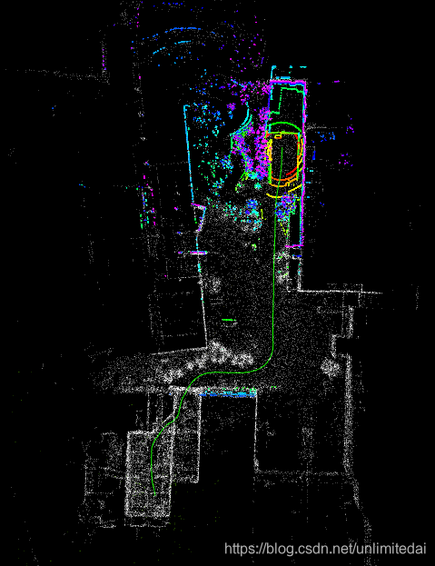
预期效果: ![一起做激光SLAM[三]位姿估计,ceres优化,地图构图](https://img-blog.csdnimg.cn/20200801115913834.gif "一起做激光SLAM[三]位姿估计,ceres优化,地图构图")
 rosbag数据: https://pan.baidu.com/s/1GaZ2eGZdfc-cluSc-bkQng 提取码: 9zsp 程序:https://gitee.com/eminbogen/one_liom
目录
点面匹配
原理
abcd点的获取
ceres优化
地图与轨迹显示
时耗与对比
时耗
与aloam对比
点面匹配
原理
对于两帧点云之间的匹配好不好,一种比较直观的体现就是位姿变换后,两帧点云完全贴合。 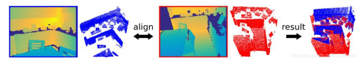 那么对于plane点来说,后一帧的某点i旋转后距离它上一帧对应的面jlm越近(h越小),那么点云就越贴合。
 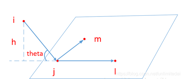 这个h的求解其实就是ij向量在平面jlm的法向量上的投影(点乘)。也就是(i-j)*法向量 我们知道平面jml的法向量求解可以使用jl和jm做叉乘实现。如下ab叉乘得到法向量。
 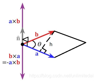 法向量也就是(l-j)×(m-j)而单位法向量要除其模 |(l-j)×(m-j)| 。 所以h=(i-j)*( (l-j)×(m-j)/法向量模 ) loam论文公式:
 ![一起做激光SLAM[三]位姿估计,ceres优化,地图构图](https://img-blog.csdnimg.cn/20200730223022442.png "一起做激光SLAM[三]位姿估计,ceres优化,地图构图") 我们使用abcd代替ijlm,写在代价函数里,代码:
我们使用abcd代替ijlm,写在代价函数里,代码:
//法向量与单位化
plane_norm = (curr_point_d_ - curr_point_b_).cross(curr_point_c_ - curr_point_b_);
plane_norm.normalize();
//h
residual[0]=abs((p_a_curr - p_b_curr).dot(plane_norm));
abcd点的获取
这里首先解释一下我们的a点是当前帧的任一点,所以整个匹配过程是将当前帧转换到前一帧贴合上,需要遍历每一个当前帧的特征点,之后再对上一帧使用KD树寻找最近点b,再根据b点上下搜索cd点,整个过程的运算量是n*n级别的,所以减少点数对时耗很重要。之所以位姿计算的是当前帧到前一帧而不是前一帧到当前帧,是因为到前一帧的位姿变换不断累积就是当前帧到最前帧也就是开始帧(世界坐标系)。 a点:直接遍历点云获取。 b点:位姿变换a点到上一帧的空间里,KD树找b点。 先把a转换到上一帧:
//用于推算一个这一帧点在上一帧lidar坐标系下的位置
void TransformToStart(PointType const *const pi, PointType *const po)
{
    Eigen::Vector3d point(pi->x, pi->y, pi->z);
    Eigen::Vector3d un_point;

    un_point= q_last_curr * point + t_last_curr;

    //输出一下
    po->x = un_point.x();
    po->y = un_point.y();
    po->z = un_point.z();
    po->r = pi->r;
    po->g = pi->g;
    po->b = pi->b;
}
利用上面的函数,laserCloudIn_plane.points[i]为a当前帧的位置,pointseed为a在上一帧的位置。
//构建一个KD树用的点,点id,点距离;将本次的a点转换到本帧下,并输入本帧全部点寻找最近点
PointType pointseed;std::vector<int> pointSearchInd;std::vector<float> pointSearchSqDis;
TransformToStart(&laserCloudIn_plane.points[i],&pointseed);
kdtreePlaneLast.setInputCloud (laserCloudIn_plane_last.makeShared());
kdtreePlaneLast.nearestKSearch(pointseed, 1, pointSearchInd, pointSearchSqDis);
kdtreePlaneLast.nearestKSearch函数,参数为 pointseed目标点(a点),1为找一个临近点(b点),pointSearchInd为临近点在输入点云(上一帧点云laserCloudIn_plane_last)里的序号,pointSearchSqDis为临近点和目标点的距离。需要多个点时会按由近到远排列顺序。 这里有一个判定,要求bcd都和a在3m内。 c点:获取b点线号,向上寻找,可以包括同线号。
//向b点的线号往上寻找c点(可以同线号)
for(int j=closestPointInd+2;(j<laserCloudIn_plane_last_num)&&(minPointInd2 == -1);j++)
{
    if(laserCloudIn_plane_last.points[j].b>closestPoint_scanID+NEARBY_SCAN) continue;
    else
    {
	double distance_a_c=(laserCloudIn_plane_last.points[j].x-pointseed.x)
			    *(laserCloudIn_plane_last.points[j].x-pointseed.x)
			    +(laserCloudIn_plane_last.points[j].y-pointseed.y)
			    *(laserCloudIn_plane_last.points[j].y-pointseed.y)
			    +(laserCloudIn_plane_last.points[j].z-pointseed.z)
			    *(laserCloudIn_plane_last.points[j].z-pointseed.z);
	if(distance_a_c>DISTANCE_SQ_THRESHOLD) continue;
	else minPointInd2=j;
    }
}
d点:向下搜索,不能同线号。
//这里不可同线号!在那个if的取并集来实现
for(int j=closestPointInd-1;(j>0)&&(minPointInd3 == -1);j--)
{
    if((laserCloudIn_plane_last.points[j].b<closestPoint_scanID-NEARBY_SCAN)||(laserCloudIn_plane_last.points[j].b==closestPoint_scanID)) continue;
    else
    {
	double distance_a_d=(laserCloudIn_plane_last.points[j].x-pointseed.x)
			    *(laserCloudIn_plane_last.points[j].x-pointseed.x)
			    +(laserCloudIn_plane_last.points[j].y-pointseed.y)
			    *(laserCloudIn_plane_last.points[j].y-pointseed.y)
			    +(laserCloudIn_plane_last.points[j].z-pointseed.z)
			    *(laserCloudIn_plane_last.points[j].z-pointseed.z);
	if(distance_a_d>DISTANCE_SQ_THRESHOLD) continue;
	else minPointInd3=j;
    }
}
ceres优化
ceres优化需要四步,构建优化的残差函数,构建优化问题,在每次获取到abcd点后添加残差块,总体优化。 构建残差函数:
//构建代价函数结构体,residual为残差。
//last_point_a_为这一帧中的点a,curr_point_b_为点a旋转后和上一帧里最近的点
//curr_point_c_为点b同线或上线号的点,curr_point_d_为点b下线号的点
//b,c,d与a点距离不超过3m
//plane_norm为根据向量bc和bd求出的法向量
struct CURVE_FITTING_COST
{
  CURVE_FITTING_COST(Eigen::Vector3d _curr_point_a_, Eigen::Vector3d _last_point_b_,
		     Eigen::Vector3d _last_point_c_, Eigen::Vector3d _last_point_d_):
		     curr_point_a_(_curr_point_a_),last_point_b_(_last_point_b_),
		     last_point_c_(_last_point_c_),last_point_d_(_last_point_d_)
	{
	    plane_norm = (last_point_d_ - last_point_b_).cross(last_point_c_ - last_point_b_);
	    plane_norm.normalize();
	}
  template <typename T>
  //plane_norm点乘向量ab为a点距面bcd的距离,即残差
  bool operator()(const T* q,const T* t,T* residual)const
  {
    Eigen::Matrix<T, 3, 1> p_a_curr{T(curr_point_a_.x()), T(curr_point_a_.y()), T(curr_point_a_.z())};
    Eigen::Matrix<T, 3, 1> p_b_last{T(last_point_b_.x()), T(last_point_b_.y()), T(last_point_b_.z())};
    Eigen::Quaternion<T> rot_q{q[3], q[0], q[1], q[2]};
    Eigen::Matrix<T, 3, 1> rot_t{t[0], t[1], t[2]};
    Eigen::Matrix<T, 3, 1> p_a_last;
    p_a_last=rot_q * p_a_curr + rot_t;
    residual[0]=abs((p_a_last - p_b_last).dot(plane_norm));
    return true;
  }
  const Eigen::Vector3d curr_point_a_,last_point_b_,last_point_c_,last_point_d_;
  Eigen::Vector3d plane_norm;
};
构建优化问题:
//优化问题构建
ceres::LossFunction *loss_function = new ceres::HuberLoss(0.1);
ceres::LocalParameterization *q_parameterization =
new ceres::EigenQuaternionParameterization();
ceres::Problem::Options problem_options;
ceres::Problem problem(problem_options);
problem.AddParameterBlock(para_q, 4, q_parameterization);
problem.AddParameterBlock(para_t, 3);
这里一定要用problem.AddParameterBlock(para_q, 4, q_parameterization);,不然优化会很奇特。。 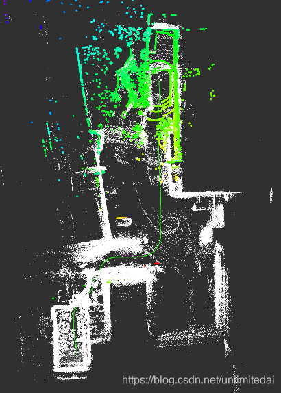 每次求出abcd点后,将他们的坐标构建成Eigen::Vector3d数据,添加残差块:
Eigen::Vector3d curr_point_a(laserCloudIn_plane.points[i].x,
			    laserCloudIn_plane.points[i].y,
			    laserCloudIn_plane.points[i].z);
Eigen::Vector3d last_point_b(laserCloudIn_plane_last.points[closestPointInd].x,
			    laserCloudIn_plane_last.points[closestPointInd].y,
			    laserCloudIn_plane_last.points[closestPointInd].z);
Eigen::Vector3d last_point_c(laserCloudIn_plane_last.points[minPointInd2].x,
			    laserCloudIn_plane_last.points[minPointInd2].y,
			    laserCloudIn_plane_last.points[minPointInd2].z);
Eigen::Vector3d last_point_d(laserCloudIn_plane_last.points[minPointInd3].x,
			    laserCloudIn_plane_last.points[minPointInd3].y,
			    laserCloudIn_plane_last.points[minPointInd3].z);
problem.AddResidualBlock(new ceres::AutoDiffCostFunction<CURVE_FITTING_COST,1,4,3>
			(new CURVE_FITTING_COST(last_point_a,curr_point_b,
			  curr_point_c,curr_point_d)),loss_function,para_q,para_t);
遍历过所有的a点后,就可以优化求解了。
//所有前一帧里的点都当a点遍历过后,进行优化
ceres::Solver::Options options;
options.linear_solver_type = ceres::DENSE_QR;
//迭代数
options.max_num_iterations = 5;
//进度是否发到STDOUT
options.minimizer_progress_to_stdout = false;
ceres::Solver::Summary summary;
ceres::Solve(options, &problem, &summary);
地图与轨迹显示
首先是位姿要累积,推算出当前帧到世界坐标系的位姿变换
//优化后,当前帧变前帧,位姿累积,并且根据位姿变换当前帧所有点到世界坐标系,放入地图中
laserCloudIn_plane_last=laserCloudIn_plane;
t_w_curr = t_w_curr + q_w_curr * t_last_curr;
q_w_curr = q_w_curr*q_last_curr ;
其次对本帧的点进行到世界坐标系的转换。
pcl::PointCloud<PointType>::Ptr laserCloud_map_curr(new pcl::PointCloud<PointType>());;
for(int i=0;i<laserCloudIn_plane_num;i=i+10)
{
    PointType point_in_map;
    TransformToMap(&laserCloudIn_plane.points[i],&point_in_map);
    laserCloud_map_curr->push_back(point_in_map);
}
之后对上面的点降采样,保存到地图里,用ros输出。
//降采样,输出地图点
pcl::PointCloud<PointType> laserCloud_map_filter;
pcl::VoxelGrid<PointType> sor;
sor.setInputCloud (laserCloud_map_curr);
sor.setLeafSize (0.2, 0.2, 0.2);
sor.filter (laserCloud_map_filter);
*laserCloud_map+=laserCloud_map_filter;

sensor_msgs::PointCloud2 laserCloudMapMsg;
pcl::toROSMsg(*laserCloud_map, laserCloudMapMsg);
laserCloudMapMsg.header.stamp = ros_cloud_plane.header.stamp;
laserCloudMapMsg.header.frame_id = "map";
pubLaserCloud_map.publish(laserCloudMapMsg);
之后是输出位姿和轨迹。
//输出位姿和path
nav_msgs::Odometry laserOdometry;
laserOdometry.header.frame_id = "map";
laserOdometry.child_frame_id = "map_child";
laserOdometry.header.stamp = ros_cloud_plane.header.stamp;
laserOdometry.pose.pose.orientation.x = q_w_curr.x();
laserOdometry.pose.pose.orientation.y = q_w_curr.y();
laserOdometry.pose.pose.orientation.z = q_w_curr.z();
laserOdometry.pose.pose.orientation.w = q_w_curr.w();
laserOdometry.pose.pose.position.x = t_w_curr.x();
laserOdometry.pose.pose.position.y = t_w_curr.y();
laserOdometry.pose.pose.position.z = t_w_curr.z();
pubLaserOdometry.publish(laserOdometry);

geometry_msgs::PoseStamped laserPose;
laserPose.header = laserOdometry.header;
laserPose.pose = laserOdometry.pose.pose;
laserPath.header.stamp = laserOdometry.header.stamp;
laserPath.poses.push_back(laserPose);
laserPath.header.frame_id = "map";
pubLaserPath.publish(laserPath);
由于有了位姿信息,所以rviz显示需要的tf可以更换为当前坐标系,这样plane,edge,ground,all_points都可以在当前坐标系下显示,刷新,一切动态了起来。
//输出世界参考系的坐标,这里transform为map_child的位姿,并在此位姿下显示当前所有点(通过 cloud_all_Callhandle函数)
static tf::TransformBroadcaster br;
tf::Transform transform;
tf::Quaternion q;
transform.setOrigin(tf::Vector3(t_w_curr.x(),t_w_curr.y(),t_w_curr.z()));
q.setW(q_w_curr.w());
q.setX(q_w_curr.x());
q.setY(q_w_curr.y());
q.setZ(q_w_curr.z());
transform.setRotation(q);
br.sendTransform(tf::StampedTransform(transform, ros_cloud_plane.header.stamp, "map", "map_child"));
这里的map是世界坐标系原点0,0,0.map_child是当前坐标系,输出点云时,当前的点plane等,frame_id要写map_child,世界坐标系,比如上面保存的地图点,在世界坐标系下显示, frame_id要写map。
时耗与对比
时耗
一开始我是保存了全部特征点(1000左右),位姿优化进行一次,每次都对当前地图点降采样,这时里程计的时耗平均是18ms,具体到每个小部分: 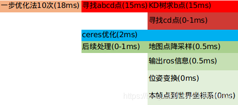 可以看出时耗基本都在复杂度n*n的KD树,将点数量降到400,两步优化,每次5迭代,只对当前帧降采样后,时耗5ms。 此时aloam的点只要384个plane点和192个左右的edge点,时耗约15-20ms。
与aloam对比
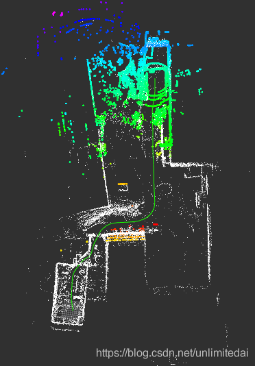
aloam只有里程计: 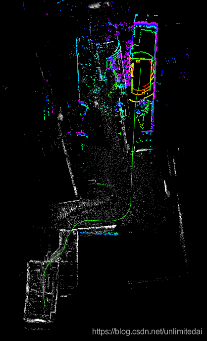 one_liom:
  aloam加上之后的地图优化: